CS111 SPRING 2010
Lecture 19: SCHEDULING AND CLOUD COMPUTING
by Ankur Gupta, Zubeen Lalani
Table of Contents
- Job Scheduling
- Disk Scheduling
- Cloud Computing Introduction
Scheduling refers to the way the available resources are distributed amongst the processes to gain required performance. The large amount of work required to be run on limited number of resources makes scheduling an important task.
Types of Operating System Schedulers
The three types of scheduling prevalent in a system are as follows:
1) Long-term Scheduling
If we were to ask,"Which processes are to be admitted into the system(to be run)?" then this is the task of the Long-term scheduler. It dictates what processes are to run on a system and the degree of concurrency to be supported at anytime. In modern operating systems, this is used to make sure that real time processes get enough CPU time to finish their task. Long term scheduling is also important in batch processing systems.
2) Medium-term Scheduling
If we were to ask, "Which processes should reside in RAM(main memory)?" then this is the task of the medium term scheduler. The processes which are in the RAM can be loaded easily. Otherwise the pages for that particular process will have to be loaded from the secondary memory. This "swap-in" and "swap-out" is done by the medium term sheduler.
3) Short-term Scheduling
If we were to ask, "Which processes have CPU?" then this is the task of the short term scheduler. It determines which available process will be executed by the processor. It is also called the dispatcher.
Scheduling Metrics<
Scheduling Metrics are used to measure how good/suitable a Scheduler is. The concept of scheduling predates computers. The time line of a job (say repairing a car at a factory) can be represented as follows
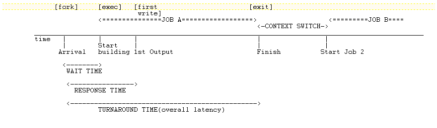 If we are using a browser then we expect it to have a low response time whereas the turn around time wont be an important metric. However in a pay roll application the turn around time is a more realistic metric. Therefore the application defines which metric is more relevant.
Aggregate Statistics:
1) Utilization: The % of the CPU time spent doing useful work.
2) Throughput: The rate at which useful work is being done.
Goals of scheduler:
1) Maximize utilization of resources
2) Minimize the average and worst-case wait times, response times, and turnaround times.
The above goals may be conflicting. A good policy maximizes fairness and maximizes throughput.
Scheduling Algorithms
1) First Come First Served (FCFS)
This algorithm performs the processes to completion, in the order of their arrival time. Consider the following example:
(assuming 1 cpu and no preepmtion)
| JOBS |
ARRIVAL TIME |
RUN TIME |
WAIT TIME |
TURNAROUND TIME |
| A |
0 |
5 |
0+d |
5+d |
| B |
1 |
2 |
4+2d |
6+2d |
| C |
2 |
9 |
5+3d |
14+3d |
| D |
3 |
4 |
13+4d |
17+3d |
The processes run by the CPU will be in the following order:
dAAAAAdBBdCCCCCCCCCdDDDD
Here each capital letter represents one clock cycle and d is the time for context switch.
Utilization = 20/(20+4d) == 1
Avg. wait time =(22+10d)/4 = 5.5 + 2.5d clock cycles
Avg. turnaround time= (42+10d)/4 = 10.5 + 2.5d clock cycles
One can see that problems arise if one of the earlier jobs has a long runtime and ties up the CPU for a long period of time before allowing later processes to perform. In the specific example given above, the average wait time could have been decreased if we had scheduled D before C.
2) Shortest Job First (SJF)
This algorithm chooses the shortest job to run whenever the decision has to be made. The shortest job will hold the CPU for less time and allows us to improve the wait time overall. The SJF algorithm my starve the longer jobs.
(assuming 1 cpu and no preepmtion)
| JOBS |
ARRIVAL TIME |
RUN TIME |
WAIT TIME |
TURNAROUND TIME |
| A |
0 |
5 |
0+d |
5+d |
| B |
1 |
2 |
4+2d |
6+2d |
| C |
2 |
9 |
9+4d |
18+4d |
| D |
3 |
4 |
4+3d |
8+3d |
The processes run by the CPU will be in the following order:
dAAAAAdBBdDDDDdCCCCCCCCC
Here each capital letter represents one clock cycle and d is the time for context switch.
Utilization = 20/(20+4d) ~= 1 //same as FCFS
Avg. wait time =(18+10d)/4 = 4.25 + 2.5d clock cycles
Avg. turnaround time= (39+10d)/4 = 9.25 + 2.5d clock cycles
Preemption : The currently running process may be interrupted and moved to the ready state by the OS. The decision to preempt may be performed when a new process arrives, when an interrupt occurs, or periodically based on clock interrupt.
Scheduling Algorithms with Preemption:
The periodic clock interrupt will allow context switching between processes. For the following examples let the quanta of time for which each process runs before it is preempeted be 1.
1) SJF+Preemption:
Consider the example we worked out for SJF. Now let us add preemption to this.
The processes run by the CPU will be in the following order:
dAdBBdDDDDdAAAAdCCCCCCCCC
Here each capital letter represents one clock cycle and d is the time for context switch.
Utilization = 20/(20+5d) ~= 1 //same as FCFS
Avg. wait time =(d+2d+9+5d+3d)/4 = 2.25 + 2.75d clock cycles
Avg. turnaround time= ((11+4d)+(3+2d)+(20+5d)+(7+3d))/4 = 10.25 clock cycles
2) FCFS +Preemption = ROUND ROBIN
The processes run by the CPU will be in the following order:
dAdBdCdDdAdBdCdDdAdCdDdAdCdDdAdCCCCC
Here each capital letter represents one clock cycle and d is the time for context switch.
Avg. wait time = order of d
Avg. turnaround time = 12.25
This new implementation decreases our average wait time to 0 but increases our average turnaround time to 12.25. These times are valid so long as the context switching time between processes d is very very less than the time between context switches.
A strong advantage to the Round Robin scheduling implementation is that it is very fair.
Real Time Scheduling
Def: Real time is not just real fast, Real time means that correctness of result depends on both functional correctness and time that the result is delivered.
Real time tasks can be classified as:
1)Hard Real Time Task: It is one that must meet its deadline.
2)Soft Real Time Task: It is one that has an associated deadline which is desirable but not mandatory.
Some algorithms for scheduling Soft Real Time tasks are:
1) Earliest Deadline First Scheduling
This algorithms simply schedules the job with the earliest deadline. If any schedule exists for a given set of real time processes, then the earliest deadline schedule for that set of processes also exists. However this algorithm is not fair. When the system is overloaded, the set of processes that will miss deadlines is largely unpredictable.
2) Rate Monotonic Scheduling
This algorithm is a scheduling algorithm used in real-time operating systems with a static-priority scheduling classes. These classes may be high, medium and low (say). This algorithm is fair as compared to Earliest Deadline First sheduling as the processes now have priorities associated with them. This scheduling type however faces the Priority Inversion bug.
Priority Inversion occurs when a low priority task holds resource that prevents execution by high-priority task.A similar bug was found in the mars rover. Check out suggested readings for more information. Consider the following scenario:
- Task 3 acquires lock
- Task 1 needs resource, but is blocked by Task 3, so Task 3 is allowed to execute
- Task 2 preempts Task 3, because it is higher priority
- BUT, now we have Task 2 delaying Task 3, which delays Task 1
To avoid this Priority Transfer is done, when a low priority thread temporarily gets a high priority at the expense of the high priority task which is waiting for the lock.
To refresh your concepts about how a disk works, take a look at the following lecture scribe notes: Hardware Review
Basically, the factors that affect the disk performance are:
1. Seek time
2. Rotational Latency
If we have multiple I/O requests available, then deciding which one to schedule first becomes important if we want to reduce the latency.
Here is a simple abstraction to see how to calculate the access time:
As is visible in the figure, the cost to reach the desired position (i) from the current read head position (h) is |i - h|.
To calculate the average seek time, we will need to use a little bit of calculus:
Average Seek Time = 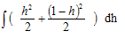 = 1/3 = 1/3
Disk Scheduling Algorithms
The two simplest disk scheduling algorithms are:
1. FCFS (First Come First Serve)
As the name suggests, it simply servers the first request in the queue.
Disadvantage:
- Large seek time as the disk head may have to jump from one extreme to another.
Advantage:
- It is fair and doesn't result into starvation.
2. SSTF (Shortest Seek Time First)
It serves the requests in the increasing order of their seek times i.e. the request with the shortest seek time is served first.
Advantages:
- Minimizes seek time
- Maximizes throughput
Disadvantages:
- Not fair. Starvation is possible.
- More CPU time required to find out the shortest seek time.
More sophisticated algorithms for disk scheduling includes:
1. Combination of FCFS and SSTF
Here, FCFS is used for scheduling the batches (of requests) and SSTF is used for scheduling within a batch. Once a batch has been scheduled to run, no other requests are allowed to be added in this batch.
Advantages:
- No starvation within a batch (using SSTF).
2. Elevator Scheduling
Just like a building elevator, it keeps moving the disk head in the same direction until there are any more requests in that direction, when it starts moving in the reverse direction.
Disadvantage:
- It is unfair, as it results into more wait for the requests at the ends (just like Boelter elevator).
3. Circular Elevator Scheduling
To overcome the unfairness inherent within Elevator algorithm, the disk head can be made to move in only one direction by getting it to magically jump to the start (of the requests) once it reaches the end (of the requests).
Advantages:
- Fair, no starvation
Disadvantage:
- Lower throughput as the disk head takes more time while it has to jump over to the starting position.
4. Anticipatory Scheduling
Suppose we have two threads A and B and they read the following disk sectors sequentially:
TA: 0,1,2,3, ....
TB: 1000000,1000001,1000002, ....
such that the requests arrive in an interleaved fashion i.e.
0,1000000,1,1000001,2,1000002
Using FCFS will results into disk head going from 0 -> 1000000 -> 1 -> 1000001 .... which will result into large seek time.
Anticipatory algorithm tries to minimize the seek time by trying to guess the future. It assumes that a new request to access a location will result into more requests in the vicinity and hence it waits for more requests to arrive for the nearby sectors (DALLYING) rather than jumping over to the next available request with a long seek time.
Advantage (as well as Disadvantage):
- Guessing can be risky. If the guess is correct, it will result into less seek time but if the guess is wrong,
it might result into wastage of waiting time.
What about FLASH drive?
Can we use the above seek time calculations and algorithms for the FLASH drive?
The answer is mostly no. As flash drive is random-access, our formula to calculate the access cost (|i - h|) fails here. So, we can't use SSTF or Elevator algorithm here. We can still use FCFS though. To minimize the latency batched requests can be used.
What is Cloud Computing?
Quoting from Wikipedia:
"Cloud computing is Internet-based computing, whereby shared resources, software and information are provided to computers and other devices on-demand, like the electricity grid."
Quoting from "Above the Clouds: A Berkeley view of Cloud Computing":
"Cloud Computing refers to both the applications delivered as services over the Internet and the hardware and
systems software in the datacenters that provide those services. The services themselves have long been referred to as
Software as a Service (SaaS). The datacenter hardware and software is what we will call a Cloud."
These days, shipping container based datacenters are in norm and they are placed near a river to reduce the cooling costs.
Advantages:
1. Large Shared Resources (Economies of Scale)
2. From a customer point of view:
- short-term commitment
- flexibility - ability to grow as needed "instantly"
- can be easily used when demand is unknown beforehand
- efficient to use for varying demand
Problems / Issues:
1. Payment: OS must meter activities in a way that both the customer and the supplier trust it.
2. Resource Management: How to manage the large number of resources available in a cloud?
3. Security and Data Confidentiality:
Standard techniques:
- encrypted connection to cloud
- encrypt all files in the cloud
4. Software Licensing Cost: E.g. Honeypot research could not be done on Windows due to huge licensing costs involved.
5. Data Transfer Bottleneck: With the advent of cloud computing, the CPU and disk resources stop being a bottleneck, but now data transfer becomes a bottleneck as the CPUs wait a long time for the input data to be copied to its disk from some other disk (which had produced that input).
6. Vendor lock-in: Once you start using the cloud services from a vendor, you can't really switch over to a different vendor as the different vendors' clouds are not compatible with each other.
In the end, TRUST is the most important factor that is blocking the organizations from using the cloud services.
Trusting trust
In "Reflections on trusting trust", Ken Thompson shows how any system in the world can be broken into.
He created a login.c program where he changes the UNIX login program and adds the following lines:
if (user == "ken")
become root;
Now, once he compiles it the object file login.o can be used to take control of any system.
To make sure, nobody can catch this bug in the code, he modifies the C compiler i.e. cc.c where he adds the following lines:
if compiling login.c
insert login bug
Again, to make sure that nobody can identify the bug in cc.c he adds two more lines:
if compiling cc.c
insert buggy code
Similarly, any program that can be used to identify these bugs can be modified to make this bug invisible. (e.g. gdb)
This shows that no system in the world is perfectly secure and it is very important to trust the people who wrote the software.
Suggested Readings
1. Mars PathFinder Account
2. Reflections on Trusting Trust - Ken Thompson's Turing Award Lecture
|