CS111 SPRING 10

Table of Contents

1. Scheduling
   1. Scheduling Metrics
   2. Simple Schedulers
      1. Example 1: First In, First Out
      2. Example 2: Shortest Job First
   3. Preemption
      1. Example 3: SJF + preemption
      2. Example 4: Round-Robin
   4. Priorities
      1. Real-Time Scheduling
      2. Priority Inversion
   5. Simple Disk Scheduler
      1. Shortest-Seek-Time-First Scheduling.
      2. First-Come, First-Served Scheduling.
      3. Chunking Algorithm.
      4. Elevator Algorithm.
      5. Cycle + Elevator Scheduling.
      6. Anticipatory scheduling.
2. Cloud Computing
3. Conclusion: TRUST!

Scheduling

In an operating system, since there are limited resources (CPU, RAM) caused by too having many users, processes, and various other tasks, we need a way to divide the resources up. This is the scheduler job, to be a "glorified bouncer" that decides when and who gets access to the CPU and/or RAM. There are three types of scheduling: long term scheduling, medium term scheduling, and short term scheduling. Long term scheduling deals with deciding which processes are admitted into the system. Medium term scheduling has to do with deciding which processes are allowed to reside storage. Preferable, processes would want to reside in RAM versus the disk because of faster memory access. Finally, short term scheduling deals with deciding which process gets the CPU. All three of these decisions are done by the scheduler.

Scheduling Metrics

To evaluate the performance of schedulers, we have the following metrics: wait time, response time, and latency. Consider the following diagram:

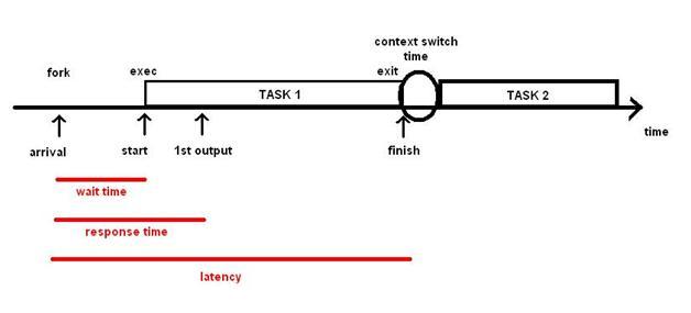
A job starts with the arrival of a request. This is analogous to a fork(). After some setup, such as identify the request and gathering the necessary resources, we finally start doing actual work [exec]. The time between the arrival and start of work is called the wait time. Next, after some time, we get the first noticeable output [first read() or write()]. The time between the arrival and first output is known as the response time. Finally, we finish the task [exit]. The time between the arrival and finish is called the turn around time (TT) a.k.a. latency. When we want to run another task, there is some setup time before we can actually start do the work [context switch]. The time between the start and finish time is considered the runtime.

The goal of any scheduler should be minimize the wait, response, and turn around times, while maximizing utilization, which is defined as the percentage of CPU time spent doing useful work, and throughput, the rate of useful work being done. However these goals sometimes conflict with each other. Thus, it is the job of the engineer to decide the tradeoffs when writing a scheduler.

Simple Schedulers

For the following scheduling algorithms, assume we have four jobs: A, B, C, and D, and we are operating with one CPU. You can find the information on each job in the following table:

JOBS	ARRIVAL TIME	RUNTIME
 A	   0		  5	
 B	   1		  2
 C	   2		  9
 D	   3		  4

Example 1: First In, First Out (FIFO)

FIFO is operates on a first come, first serve basis, that is whoever arrives earliest, gets to perform and finish their work before those that arrive after. If we use FIFO as our scheduler, we get the following scheduling order along the time axis:

||AAAAA||BB||CCCCCCCCC||DDDD
Note that || refers to a context switch time

Since A arrived first, it gets the CPU and runs for five seconds before it finishes. While A runs, B, who arrived at time 1, has to wait for A to finish before it can start doing work. B's wait time is 4 seconds. similarly, even though C arrived at time 2, it has to wait for both A and B to finish before getting access to the CPU. For D, it has to wait for A, B, and C. The following is summary of the wait times. For simplicity, context switch times have been omitted.

JOBS	WAIT TIME
 A	   0 
 B	   4
 C	   5
 D	   13

Notice that the utilization is roughly equal to 1 or 100% (ignoring the context switching)
average wait time = 5.5
average turnaround time = 10.5.

In FIFO, notice that D has to wait for a very long time. In addition, D can starve and never run if C runs forever. In actuality, any of the jobs that arrive after A will starve with A runs indefinitely.

Example 2: Shortest Job First (SJF)

SJF schedules based on the following statement, "When it is time to run a job, run the shortest job first." Using the same example, we seen that under SJF we have the following run order

||AAAAA||BB||DDDD||CCCCCCCCC

Thus, we get the following wait times:

JOBS	WAIT TIME
 A	   0 
 B	   4
 C	   9
 D	   4

average wait time = 4.25
average turnaround time = 9.25
Notice that D has considerable less wait time when compared to FIFO.

In SJF, a long job can starve and never be allowed to run if shorter jobs are constantly added. In addition, SJF requires knowledge of a jobs runtime, which cannot always be determined with great accuracy.

Preemption

To avoid potential starvation, preemption is used. After a certian amount of time, a clock interrupt occurs and the scheduler is automatically called and determines who gets to run next. For the following example, we assume that a clock interrupt occurs every one second.

Example 3: SJF + preemption

With this scheduling algorithm, we get the follow job order:

||A||BB||DDDD||AAAA||CCCCCCCCC

JOBS	WAIT TIME
 A	   0 
 B	   0
 C	   9
 D	   0

average wait time = 2.25
average turnaround time = 8.75

Notice how C is the only one that waits, very UNFAIR!!!! Thus, we establish fairness metrics, such as worst case wait time and worst case run time. We must also consider these fairness metrics when writting scheduling algorithms. The standard deviation of these times is also another option to consider.

Example 4: Round-Robin (RR)

RR is essentially FIFO with preemption. Thus, the job order is as follows:

||A||B||C||D||A||B||C||D||A||C||D||A||C||D||A||CCCC

JOBS	WAIT TIME
 A	   0 
 B	   0
 C	   0
 D	   0

average wait time = 0
average turnaround time = 12.25

Although the average wait time is now roughly zero, the average turnaround time increased. In addition, RR has many context switches. We have been assuming context switches = 0, as this is a pretty good assumption when considering the CPU. However, if we consider a disk drive, context switching is expensive. Thus, RR might not be the best choice in that situation. More can be found on disk scheduling later.

Priorities

In the previous scheduling examples, there has been a set of rules that we consider to determine who runs first. These rules determine the priority of a job. In FIFO, priority is determined by arrival time. Similarly for SJF. priority is determined by runtime. Priorities are set by the user, particularly in real-time applications, or by the system.

Real-Time Scheduling

In real-time applications, there are some constraints and deadlines that must be done or hit, or else DISASTER!! This type of scheduling is called hard realtime. Examples of these high priority tasks include car brakes and nuclear power plant reactors. On the other side, there are some tasks with low priority such as a frame when video streaming. This type of scheduling is called soft realtime. If a deadline is missed, we just drop the task. To possible implementations of soft realtime are easilest meetable deadline first and rate-monatomic scheduling. In easilest meetable deadline first, highest priority is given to tasks that the "easiest," generally those that has the shortest runtime. For rate-monatomic scheduling, let's consider a case where we want to stream ten videos at the same time with 20 frames/sec (security guard monitoring), but we do not have the CPU capacity to run at that level. With rate-monatomic, the scheduler with notice this and start stream all 10 videos at reduced performance, let's say 15 frames/sec.

Priority Inversion

Let's consider the example of the Mars Rover. The Rover has three levels of priority with blocking mutexes: low, medium, and high. The low priority task started and locked the data. Before the low priority thread unlocked, a high priority task, which tries to acquire the same lock that the low priority has, and a medium priority task starts. Since the low has the lock, the high waits for the low, but since the medium has higher priority than the low, the medium takes control and runs. The medium runs forever, and thus, the high priority task never runs.
To solve this problem, we use priority inversion, where the high priority task temporarily upgrades the priority of the low task to have high priority. Thus, the low finishes, the high runs, and then the medium runs, avoiding the deadlock and potential DISASTER!!

Simple Disk Scheduler

Imagine we have 1 CPU and 1 Harddisk with many I/O request. Which I/O request should we do first? If requests are scattered throughout the harddisk, we need an algorithm that efficiently minimizes the seek time and rotational latency.

The simple diagram shows the

Cost to Access = | i - h |

where i = desired action and h = read head

The disk controller serves one request at a time. Any other additional requests, normally from other processes, will need to be queued. Given that we want access the whole bunch of blocks: { }, how do we schedule the access order to optimize seek time?

Shortest-Seek-Time-First Scheduling. (SSTF)

Method: Select the request with the minimum seek time from the current head position. This means the disk controller services together all requests close to the current head position, before moving the head far away to service another request.

Advantages:
+ minimizes seek time
+ maximizes throughput

Disadvantage:
- more CPU time
- STARVATION

First-Come, First-Served Scheduling. (FCFS)

Method: Selecting the request in the order they arrive.

Advantages:
+ no starvation
+ easy to program

Disadvantage:
- cannot optimize seek time
Given random requests, the average seek time is |R-H|.

( LOOK CALCULUS! )

Chunking Algorithm. (FCFS + SSTF)

Method: Grab a batch of 10 elements, do SSTF on these 10 elements before batching the next 10 elements.

Advantages:
+ no starvation
+ increase batch size for performance
+ decrease batch size for fairness

Elevator Algorithm.

Method: Keep moving in the same direction until there are no more outstanding requests in that direction, then they switch directions. (SSTF in a positive Direction)

Advantages:
+ no starvation

Disadvantage:
- Avg Wait Time for Ends are Longer
The average wait time in the middle is t/2.
The average wait time at the top or bottom is t/4.

Cycle + Elevator Scheduling.

Method: Keep moving in the same direction until there are no more outstanding requests in that direction, and then starts back in the beginning.

Advantages:
+ no starvation
+ The average wait time is t/2 everywhere.

Anticipatory scheduling.

Method:Suppose we have two processes A and B, each reads disk sequentially.
A: 0, 1, 2, 3, ....
B: 10000, 10001, 10002, 10003, ....

A process appears to be finished reading from the disk when it is actually processing data in preparation of the next read operation. This will cause switching to an unrelated process.
The request order using SSTF: 0, 10000, 1, 10001, 2, 10002
You can see there is a lot of Seeking. Anticipatory scheduling waits for a short time after a read operation in anticipation of another close-by read requests.

Advantages:
+ minimize seeks by guessing future request
+ Dallying!

Cloud Computing

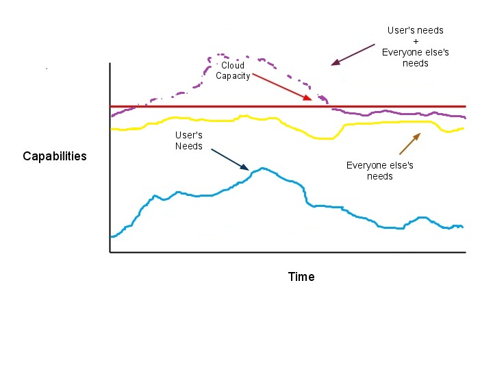
Cloud Computing is a paradign shift from service delivered from mainframes held within the company to services delivered by clusters in data centers. The term "cloud" is a metaphor for the internet as an abstraction of the underlying infrastructure it represents.

Advantages:
+ Large shared resources
+ Economy of scale
+ Short-term commitment
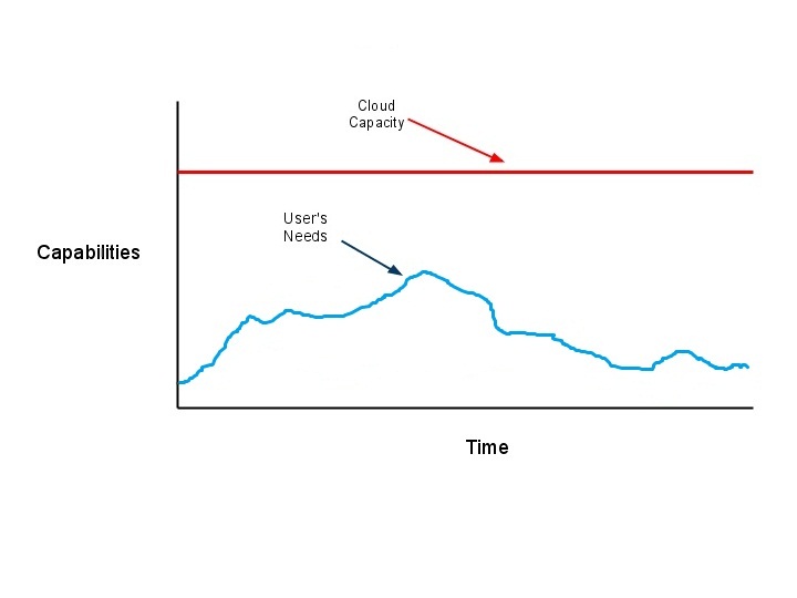
+ Can grow as needed
+ Able to handle Unknown/Varying demand

Disadvantages:
- Payment - (OS must meter activites) - Trust
- Resource Managment
- Data confidentiality
- Encryption Needed - Both File and Connection
- Software lincesing
- Data transfer bottlenck

Conclusion: TRUST!

From an Operating Systems viewpoint, Operating Systems do not trust applications because they don't trust the user and the programmers behind it. But what about the Operating System itself?

Kent Thompson wrote a paper, Reflections on Trusting Trust that revealed we cannot always trust even simple login.

login.c:

(if user == "kent")

Become Root

But this can be easily detected by going through the c code!

So change the Object Code! login.o
Or better yet, change the Compiler!

gcc.c:

if (compiling "login")

insert above login.c code;

if (compiling "gcc")

insert the whole code!

In the end, you have to just trust them!